Part 2: Identifying specific objects in the population

Now that we know how to simulate populations of binaries, let’s think about how we can identify specific objects in the population. Again, we’ll start with a demo from Tom and then give you some tasks to work on.

Demo

Let’s make a slightly larger population so that our plots look a little nicer.

p = cogsworth.pop.Population(
    n_binaries=10000,
    use_default_BSE_settings=True
)
p.create_population()

Inspect initial conditions

We’ve also explored some of the output tables already, including the initial_binaries table that contains the initial conditions for each binary. Let’s quickly plot the initial component masses of the binaries.

fig, ax = plt.subplots()
ax.scatter(p.initial_binaries["mass_1"], p.initial_binaries["mass_2"], s=1)
ax.set(
    xscale="log",
    yscale="log",
    xlabel="Initial primary mass, $M_{1, i}$ [M$_\odot$]",
    ylabel="Initial secondary mass, $M_{2, i}$ [M$_\odot$]",
)
plt.show()

In COSMIC, by default there’s a lower limit on the initial secondary mass such that its pre-main-sequence lifetime is not longer than the main sequence lifetime of the primary. This is why there’s a cutoff of objects in the lower right of the plot.

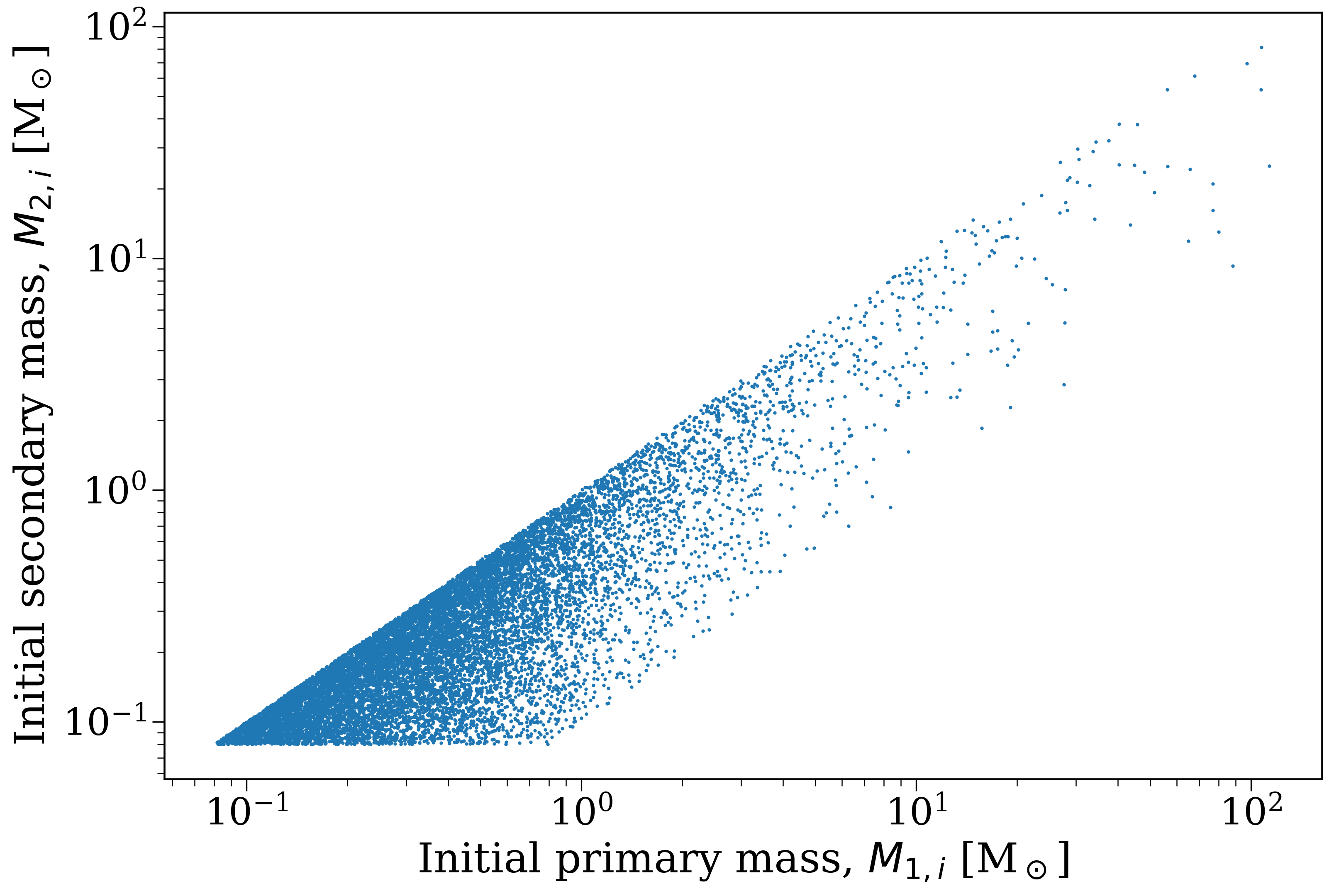
Initial component masses of all binaries in the population.

By definition, the initial primary mass is always greater than or equal to the initial secondary mass, so all of the binaries lie below the diagonal line in this plot. But there’s a variety of mass ratios shown. Let’s consider a scenario where we only care about binaries with mass ratios that are far from unity. We can create a mask to select only those binaries.

Mask based on initial conditions

In the case where we only care about systems where \(q \equiv M_{2, i} / M_{1, i} < 0.5\), we can create a mask like this:

mass_ratio_mask = (p.initial_binaries["mass_2"] / p.initial_binaries["mass_1"]) < 0.5

As we discussed in the last part, each binary in a population is assigned a unique binary number (bin_num) that allows us to track it through the various output tables. We can use the mask we just created to get a list of the binary numbers that satisfy our mass ratio condition:

selected_bin_nums = p.bin_nums[mass_ratio_mask]
print(selected_bin_nums)

Using this mask to separate out a new population of binaries is straightforward:

# mask with bin_nums
new_pop = p[selected_bin_nums]

We can actually skip the intermediate step of getting the binary numbers and just use the mask directly to create a new population:

# mask with boolean array with same length as p.bin_nums
new_pop = p[mass_ratio_mask]

Now, if we print out the initial mass ratios for this population, we’ll see it matches our mask:

# how many binaries met this?
print(len(new_pop))

# range of mass ratios in this population
q = new_pop.initial_binaries["mass_2"] / new_pop.initial_binaries["mass_1"]
print(q.max())

Mask based on final state

We don’t just have to use the initial conditions to create masks. We can use anything that allows us to select specific bin_num values. For example, we could select only binaries that produce at least one white dwarf at the end of the simulation.

To do this, we can create a mask based on the final_bpp table, which contains the final state of every binary. This table has a column for each star in the binary (kstar_1 and kstar_2) that gives the final stellar type. White dwarfs are either kstar == 10 (helium white dwarf), kstar == 11 (carbon-oxygen white dwarf), or kstar == 12 (oxygen-neon white dwarf). So we can create a mask like this:

primary_ends_as_wd = p.final_bpp["kstar_1"].isin([10, 11, 12])
secondary_ends_as_wd = p.final_bpp["kstar_2"].isin([10, 11, 12])
has_a_wd = primary_ends_as_wd | secondary_ends_as_wd

And converting this into a new population works just like before:

wd_pop = p[has_a_wd]
print(wd_pop)
print(wd_pop.final_bpp.head())

---

Task(s)

And back to you! Here are some tasks to work on to practice identifying specific objects in the population.

Initial conditions of mergers

I’d recommend a log-scale for both the mass and orbital period!

Task 2.1.1

First, make a plot of the initial orbital period vs the initial primary mass for all binaries in the population.

Hint

The initial orbital period is given by the porb column in the initial_binaries table. You can access this table with p.initial_binaries.

Click here to reveal the answer

fig, ax = plt.subplots()
ax.scatter(p.initial_binaries["porb"], p.initial_binaries["mass_1"])
ax.set(
    xscale="log",
    yscale="log",
    xlabel="Initial orbital period, $P_i$ [days]",
    ylabel="Initial primary mass, $M_{1, i}$ [M$_\odot$]",
)
plt.show()

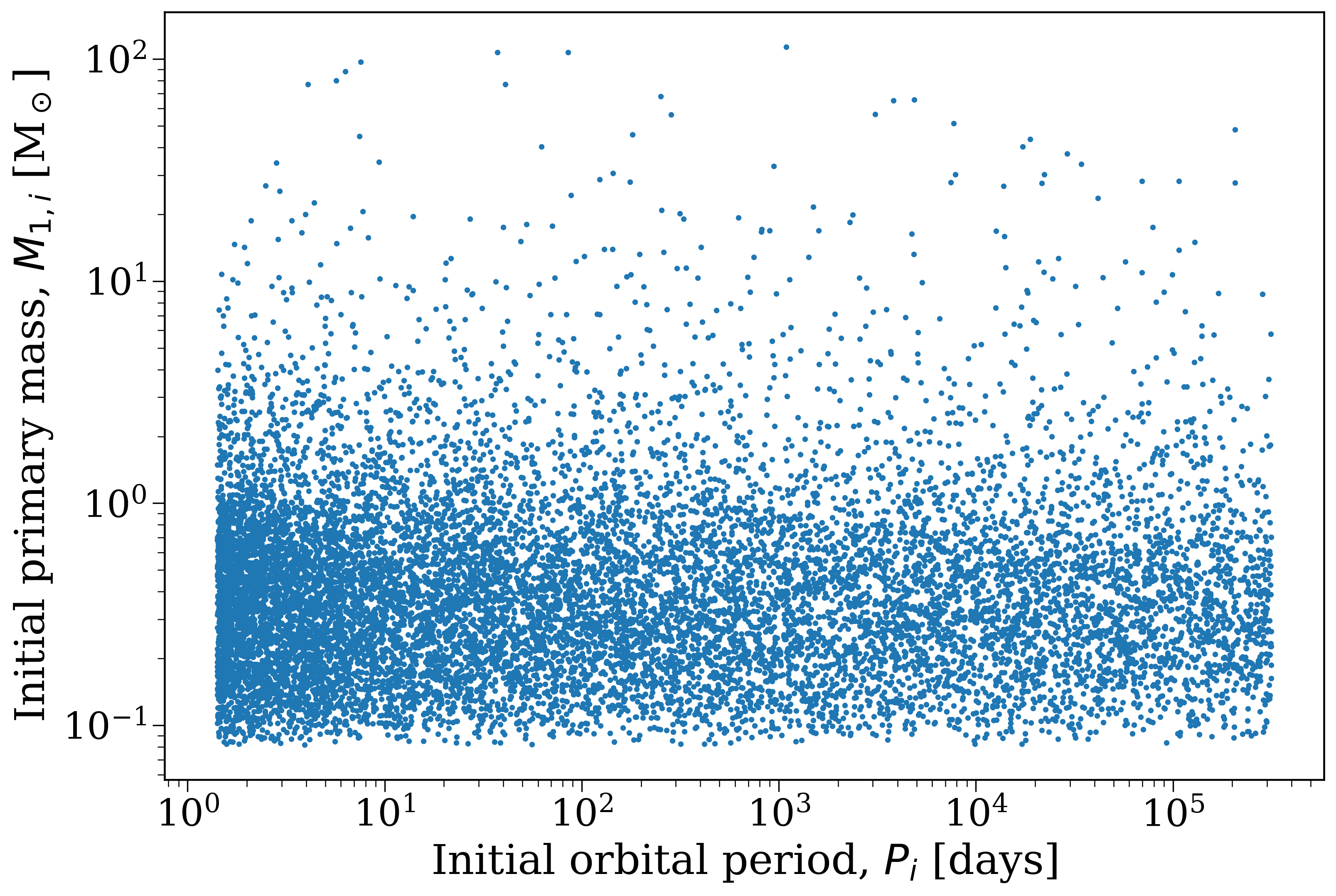
Initial orbital period vs initial primary mass for all binaries in the population.

Task 2.1.2

Now, create a mask that selects only binaries that will eventually merge (i.e. that end with a separation of exactly \(a = 0.0 {\rm R_\odot}\)).

Hint

The final separation is given by the sep column in the final_bpp table. You can access this table with p.final_bpp.

Click here to reveal the answer

merger_nums = p.final_bpp["bin_num"][p.final_bpp["sep"] == 0]
merger_mask = np.isin(p.bin_nums, merger_nums)

Task 2.1.3

Now, update your plot to highlight the binaries that will eventually merge (however you like, outline the merger points, or just overplot them in a different color, etc).

Click here to reveal the answer

fig, ax = plt.subplots()
ax.scatter(p.initial_binaries["porb"], p.initial_binaries["mass_1"], label="All binaries")
ax.scatter(
    p.initial_binaries["porb"][merger_mask],
    p.initial_binaries["mass_1"][merger_mask],
    s=50, edgecolor="darkblue", linewidth=3, facecolor="none", label="Mergers"
)
ax.legend()
ax.set(
    xscale="log",
    yscale="log",
    xlabel="Initial orbital period, $P_i$ [days]",
    ylabel="Initial primary mass, $M_{1, i}$ [M$_\odot$]",
)
plt.show()

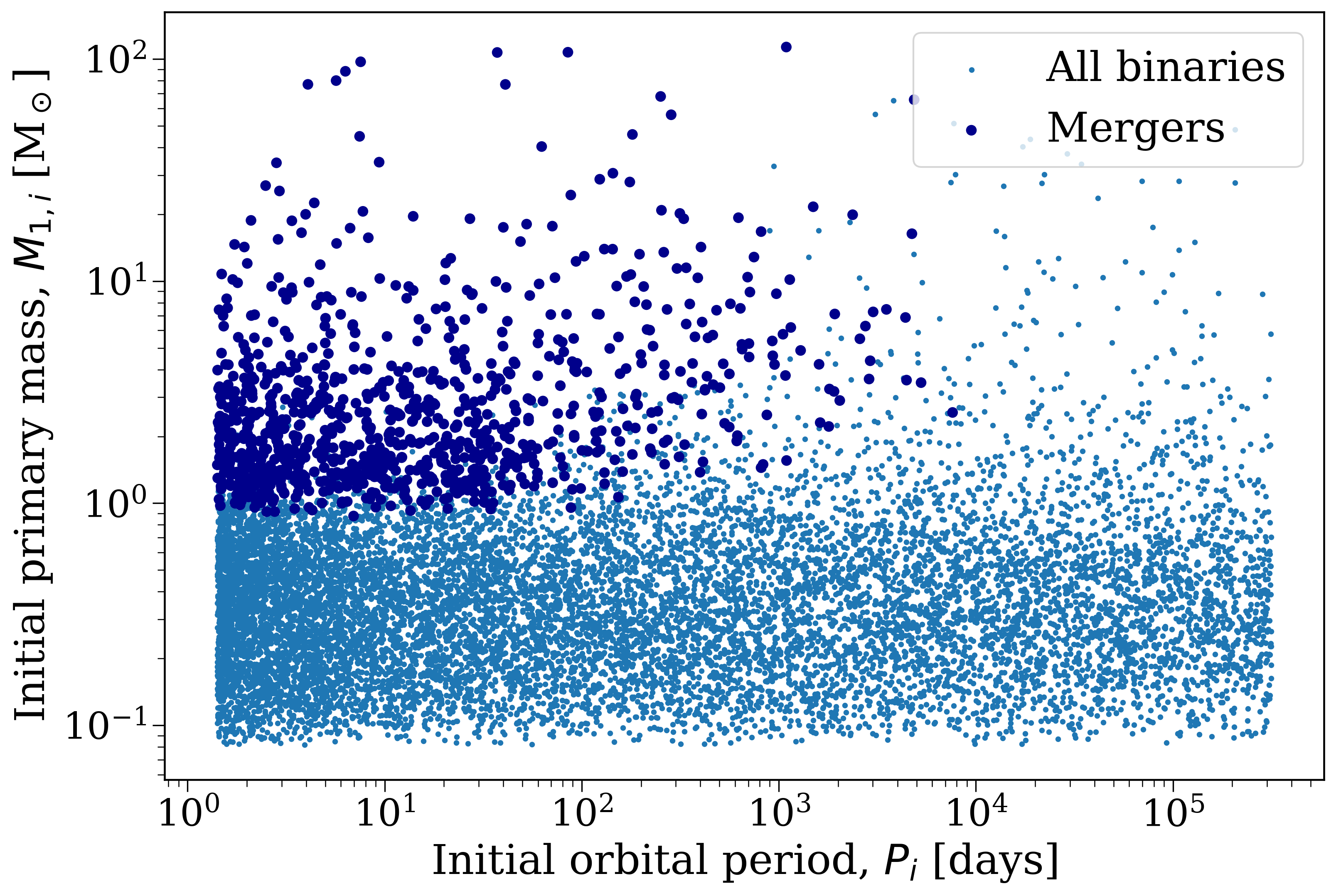
Initial orbital period vs initial primary mass, with mergers highlighted.

Task 2.1.4

What trends do you notice in your plot? Which conditions seem to lead to mergers? Why?

Click here to reveal the answer

Mergers are most common for short initial orbital periods, which makes sense since these binaries are more likely to interact and merge. Mergers are also more common for higher initial primary masses, which also makes sense since these stars are (a) larger and (b) more likely to evolve off the main sequence and expand further, leading to interactions and mergers.

[Bonus] Final positions of compact objects

If you’ve still got time, let’s try something else!

Task 2.2.1

First, make a plot of the final positions of the primary star from each binary in the population. Plot the Galactocentric radius (\(R = \sqrt{x^2 + y^2}\)) on the x-axis and the absolute Galactocentric height (\(|z|\)) on the y-axis. I recommend using a log-scale for both axes.

Hint

The final positions are given by p.final_primary_pos. This is a 2D array where the first dimension corresponds to the binary number and the second dimension corresponds to the x, y, and z coordinates.

Click here to reveal the answer

R = np.sqrt(p.final_primary_pos[:, 0]**2 + p.final_primary_pos[:, 1]**2)
abs_z = np.abs(p.final_primary_pos[:, 2])

fig, ax = plt.subplots()
ax.scatter(R, abs_z, s=1)
ax.set(
    xscale="log",
    yscale="log",
    xlabel="Final primary Galactocentric $R$ [kpc]",
    ylabel="Final primary Galactocentric $|z|$ [kpc]",
)
plt.show()

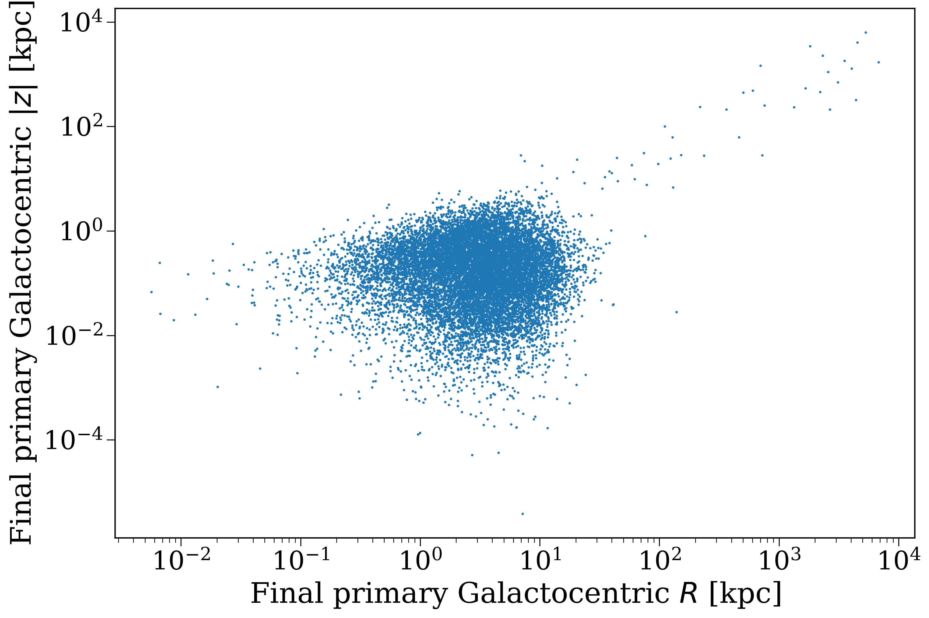
Final Galactocentric positions of the primary stars in the population.

Task 2.2.2

Now, create a mask that selects only binaries where either star ends as a neutron star or black hole (i.e. that receive a natal kick).

Hint

The final stellar type is given by the kstar_1 and kstar_2 columns in the final_bpp table. You can access this table with p.final_bpp. Neutron stars are kstar == 13 and black holes are kstar == 14.

Click here to reveal the answer

compact_object_mask = p.final_bpp["kstar_1"].isin([13, 14]) | p.final_bpp["kstar_2"].isin([13, 14])

Task 2.2.3

Now, update your plot to highlight the binaries where the primary star ends as a neutron star or black hole.

Click here to reveal the answer

fig, ax = plt.subplots()
ax.scatter(R, abs_z, label="All primaries", s=1)
ax.scatter(
    R[compact_object_mask],
    abs_z[compact_object_mask],
    s=5, edgecolor="darkblue", linewidth=3, facecolor="none", label="NS/BH"
)
ax.legend()
ax.set(
    xlabel="Final primary Galactocentric $R$ [kpc]",
    ylabel="Final primary Galactocentric $|z|$ [kpc]",
)
plt.show()

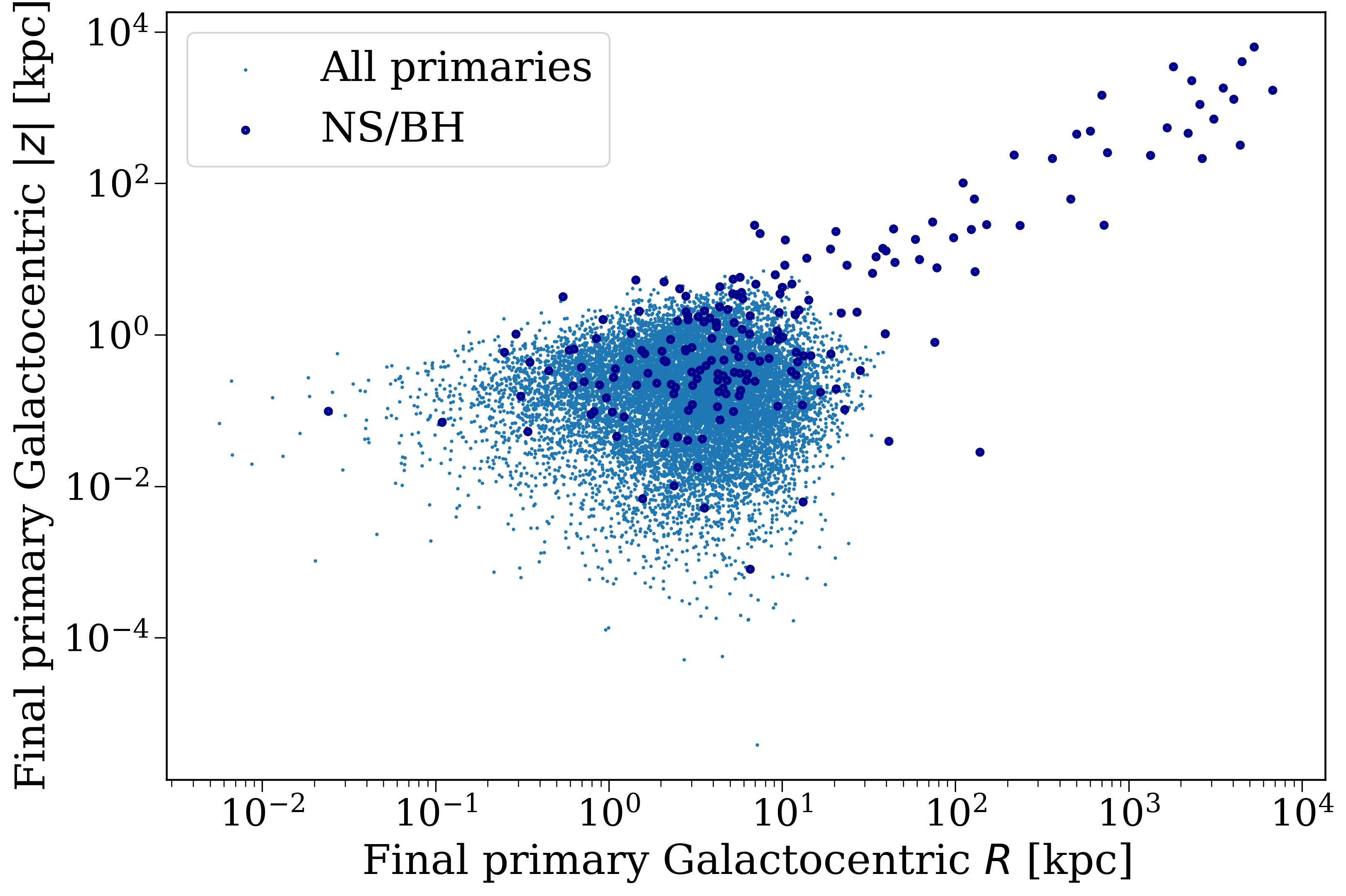
Final Galactocentric positions of the primary stars in the population, with neutron stars and black holes highlighted.

Task 2.2.4

What trends do you notice in your plot? Do the compact objects seem to have different final positions than the rest of the population? Is that true for all of them? Why/why not?

Click here to reveal the answer

The compact objects should have a wider distribution in both R and z than the rest of the population, since they receive natal kicks that can send them to different locations in the galaxy. However, this is not true for all of them. Some compact objects will still end up on similar orbits if their receive small kicks (e.g. from full-fallback black hole formation).

You could probably investigate this by colouring the points by neutron star and black hole separately if you’re interested!

And that’s it for this part! In the next part, we’ll see how we can use cogsworth to track the timing and location of supernovae in a galaxy. See you there!