Part 3: Investigate the supernovae

Now that we can simulate Populations of binaries and identify specific subpopulations, it’s time to track down those supernovae! I’ll start with a demo of how to do this and then you can do the same thing with common-envelope events.

Demo

Create a population with lots of massive stars

First things first, let’s make a slightly different population, which preferentially samples higher mass binaries. This will give us more supernovae to work with.

Note that this population still stores the total mass in binaries and singles stars required to create this population (in the mass_binaries and mass_singles attributes). So you can renormalise without worrying that you’ve preferentially sampled from the IMF.

import cogsworth

p = cogsworth.pop.Population(
    n_binaries=10_000,
    use_default_BSE_settings=True,
    final_kstar1=[13, 14],          # aim to sample systems that produce a NS/BH
    final_kstar2=[13, 14],          # same for secondary star
)
p.create_population()

Find the supernovae

Our goal here is to find the times at which supernovae occur in our population. The table of interest in this case is the bpp table, which tracks the properties of each binary at every “important” time step in the simulation.

Tip

The output documentation has a detailed description of (a) what different evol_type and kstar values mean and (b) definitions of every column in the bpp table. I recommend keeping this documentation open as you work through this part of the lab.

Supernovae are indicated by an evol_type value of 15 for primary stars and 16 for secondary stars. Any row with this value corresponds to a supernova. Let’s find these rows!

# find the rows at which a supernova occurs
primary_sn = p.bpp["evol_type"] == 15
secondary_sn = p.bpp["evol_type"] == 16
sn_mask = primary_sn | secondary_sn

# mask the rows in the Pandas DataFrame
primary_sn_rows = p.bpp[primary_sn]
secondary_sn_rows = p.bpp[secondary_sn]

Inspect supernova timing in the frame of the binary

We can now take a look at the distribution of times at which these events occur.

# use the same bins for both histograms to make it easier to compare
bins = np.linspace(0, 200, 40)

fig, ax = plt.subplots()

# plot both as density distributions
ax.hist(p.bpp["tphys"][primary_sn], bins=bins, density=True, label="Primary SN")
ax.hist(p.bpp["tphys"][secondary_sn], bins=bins, alpha=0.7, density=True, label="Secondary SN")
ax.set(
    xlabel="Time in frame of binary, $t_b$ [Myr]",
    ylabel=r"${\rm}dN/{\rm d}t_b$",
)
ax.legend()
plt.show()

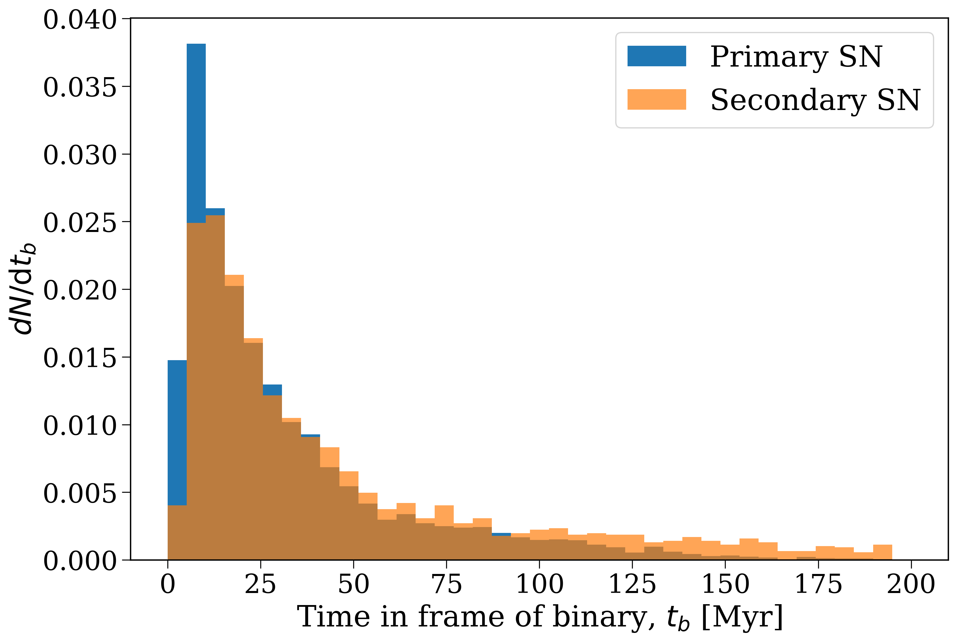
Distribution of supernova times in the frame of the binary, with primary and secondary supernovae shown separately.

It’s important to note here that these times are in the frame of the binary, so they don’t correspond to any particular time in the galaxy. We’ll see how to convert these to galactic times next.

Question for you

Why are the supernovae times different for primary and secondary stars?

Click here to reveal the answer

The timing of primary and secondary supernovae is slightly different. Primary supernovae typically occur earlier than secondary supernovae. This is because the primary star is initially more massive and therefore evolves faster, so it reaches the end of its life and explodes as a supernova before the secondary star does. The secondary star may also be affected by mass transfer from the primary, which can alter its evolution and delay its supernova explosion.

Compute the timing on Galactic timescales

Now let’s try converting these times to the galactic frame. Each binary was born at a specific time in the galaxy, which is given by the tau attribute of the initial_galaxy object. Keep in mind that this is a “lookback time”, so the binary was born \(\tau\) Myr before the present day. So to convert the supernova times to the galactic frame, we can do the following:

\[t_{\rm gal} = t_{\rm present} - \tau + t_{\rm sn}\]

where \(t_{\rm sn}\) is the time of the supernova in the binary frame and \(t_{\rm present}\) is the present day time in the galaxy (which is 12 Gyr by default, but is stored in the max_ev_time attribute).

Let’s try computing the times of the supernovae in the galactic frame!

# get the bin_nums of the supernova events
primary_sn_bin_nums = p.bpp["bin_num"][primary_sn]
secondary_sn_bin_nums = p.bpp["bin_num"][secondary_sn]

# get the indices of these bin_nums in the p.bin_nums array
primary_sn_indices = np.searchsorted(p.bin_nums, primary_sn_bin_nums)
secondary_sn_indices = np.searchsorted(p.bin_nums, secondary_sn_bin_nums)

# use these indices to get tau
primary_sn_tau = p.initial_galaxy.tau[primary_sn_indices]
secondary_sn_tau = p.initial_galaxy.tau[secondary_sn_indices]

# compute the galactic times
primary_sn_t_gal = p.max_ev_time - primary_sn_tau + p.bpp["tphys"][primary_sn].values * u.Myr
secondary_sn_t_gal = p.max_ev_time - secondary_sn_tau + p.bpp["tphys"][secondary_sn].values * u.Myr

Now let’s take a look at a plot of this

# use the same bins for both histograms to make it easier to compare
bins = np.linspace(0, 12, 20)

fig, ax = plt.subplots()

# plot both as density distributions
ax.hist(primary_sn_t_gal.to(u.Gyr).value, bins=bins, density=True,
        label="Primary SN")
ax.hist(secondary_sn_t_gal.to(u.Gyr).value, bins=bins, alpha=0.7,
        density=True, label="Secondary SN")
ax.set(
    xlabel=r"Age of Milky Way at SN, $t_{\rm gal}$ [Gyr]",
    ylabel=r"${\rm}dN/{\rm}dt_{\rm gal}$",
)
ax.legend()
plt.show()

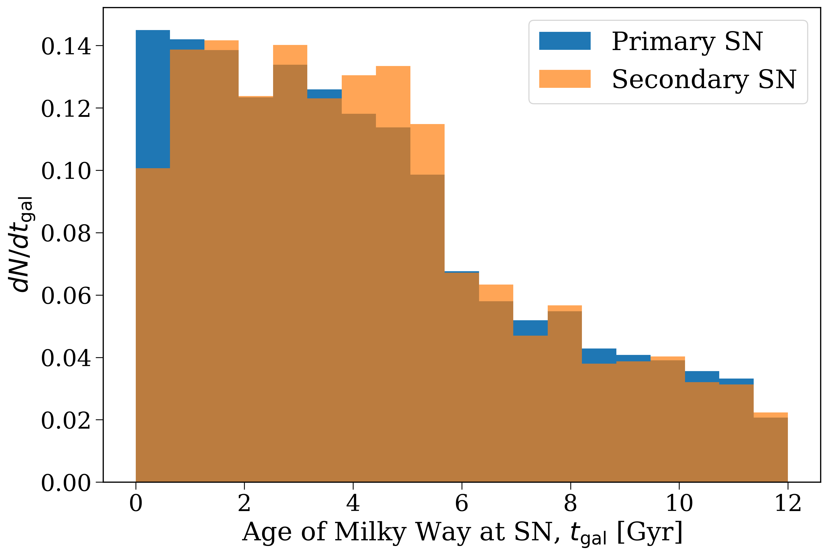
Distribution of supernova times in the frame of the galaxy, with primary and secondary supernovae shown separately.

Question for you

What drives the distribution of timing of these supernovae on Galactic timescale?

Click here to reveal the answer

The distributions of primary and secondary supernovae on galactic timescales are quite similar. Most of the supernovae (both primary and secondary) occur on short times in the context of the galaxy, so the main driver of the distribution on galactic timescales is the star formation history of the galaxy.

Locate the supernovae in the galaxy

As we’ve seen before, each binary has an orbit associated with it, which tracks its trajectory through the galaxy. Let’s take a look at one of these objects to get a sense of what a gala Orbit object looks like.

# let's take the first orbit
orbit_example = p.orbits[0]
print(orbit_example)

# it stores the time and position at each timestep
print(orbit_example.t)
print(orbit_example.pos.xyz)

Did you notice that the orbit times end at 12 Gyr? The initial time of the orbit is actually the birth time of the binary in the galaxy, these orbit times are already based in the Galactic frame.

Another complication is that the binary may have disrupted due to a supernova kick, so the secondary may be on a different orbit. cogsworth handles this and you can use p.primary_orbits and p.secondary_orbits to get the orbits of the primary and secondary stars, respectively, at every time step. So make sure to use the correct one for each supernova!

So we need to:

• Go through each of the supernovae

• Find the corresponding orbit

• Compute the last timestep just before the supernova

• Get the position of the binary at this time

Let’s do it!

primary_sn_positions = np.zeros((len(primary_sn), 3)) * u.kpc
secondary_sn_positions = np.zeros((len(secondary_sn), 3)) * u.kpc

for i in range(len(primary_sn_indices)):
    # find the corresponding orbit
    primary_sn_orbit = p.primary_orbits[primary_sn_indices[i]]

    # compute the last timestep where orbit.t is less than primary_sn_t_gal[i]
    closest_time_index = np.where(primary_sn_orbit.t < primary_sn_t_gal[i])[0][-1]

    # get the position of the binary at this time
    primary_sn_positions[i] = primary_sn_orbit.pos.xyz[:, closest_time_index]

# same for secondaries
for i in range(len(secondary_sn_indices)):
    secondary_sn_orbit = p.secondary_orbits[secondary_sn_indices[i]]
    closest_time_index = np.where(secondary_sn_orbit.t < secondary_sn_t_gal[i])[0][-1]
    secondary_sn_positions[i] = secondary_sn_orbit.pos.xyz[:, closest_time_index]

And now we can plot the positions of these supernovae in the galaxy!

fig, axes = plt.subplots(2, 1, figsize=(8, 9), gridspec_kw={"height_ratios": [1, 4]})
for pos, times in zip(
    [primary_sn_positions, secondary_sn_positions],
    [primary_sn_t_gal, secondary_sn_t_gal],
):

    XMAX = 30
    ZMAX = 7.5

    axes[0].scatter(
        pos[:, 0], pos[:, 2],
        c=times.to(u.Gyr).value, s=5,
        cmap="magma", vmin=0, vmax=12
    )

    axes[1].scatter(
        pos[:, 0], pos[:, 1],
        c=times.to(u.Gyr).value, s=5,
        cmap="magma", vmin=0, vmax=12
    )
axes[0].set(
    ylabel="$z$ [kpc]",
    xlim=(-XMAX, XMAX),
    ylim=(-ZMAX, ZMAX),
    aspect="equal",
)
axes[1].set(
    xlabel="Galactocentric $x$ [kpc]",
    ylabel="Galactocentric $y$ [kpc]",
    xlim=(-XMAX, XMAX),
    ylim=(-XMAX, XMAX),
    aspect="equal",
)

fig.colorbar(axes[0].collections[0], ax=axes, label="Age of Milky Way at SN [Gyr]")

plt.show()

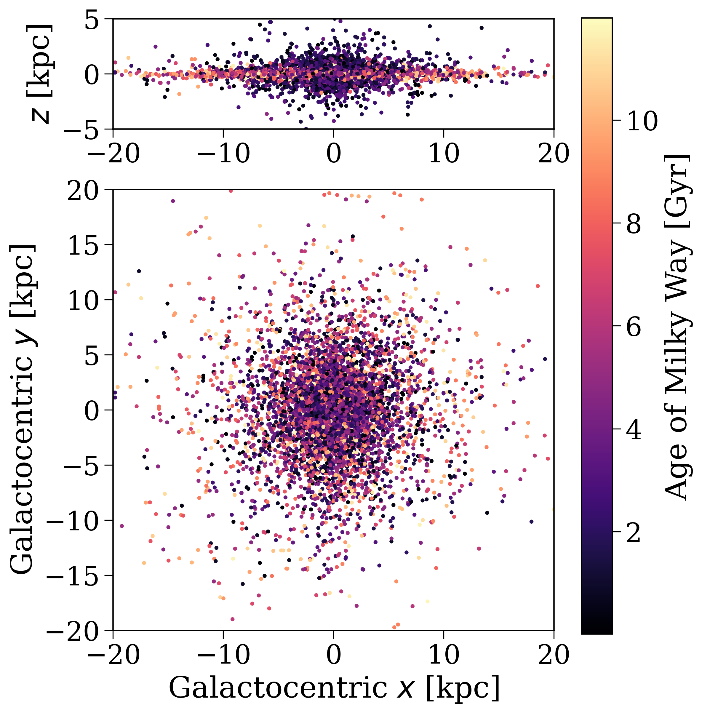
Positions of supernovae in the galaxy. The colour indicates the age of the Milky Way at which the supernova occurs.

---

Tasks

Now it’s your turn to do the same for common-envelope events! The code from the demo above should be helpful for this :)

You can also imagine that simulating the location of NS-NS mergers in the galaxy would be important for understanding the chemical enrichment from these events, since they are important sites of \(r\)-process nucleosynthesis. The trouble is that these are so rare that simulating enough of them to get a good picture of their distribution in the galaxy would require a much larger population than we can simulate in the time we have here.

Why care about the location of common-envelope events?

This lab is for a nucleosynthesis workshop, so it should be immediately obvious why we spent some time thinking about where supernovae occur in the galaxy - the chemical enrichment from these events will depend on where they occur. But common-envelope events are _also_ important for nucleosynthesis! They lead to the formation of NS-NS binaries which are important sites of \(r\)-process nucleosynthesis and can lead to type Ia supernovae which produce nickel.

So if you’re interested in learning about the chemical enrichment - understanding where common-envelope events occur in the galaxy is also important!

Task 3.1

Create a population like the one above (~10000 binaries, that preferentially samples higher mass binaries). Write a mask for the bpp table that selects only the rows corresponding to common-envelope events. It may be useful to know that common-envelope events are labelled as evol_type == 7.

Hint

Common-envelope events aren’t specific to an individual star, so you don’t need to keep primary and secondary events separate here, you can just make one mask for all common-envelope events.

Click here to reveal the answer

import cogsworth

p = cogsworth.pop.Population(
    n_binaries=10_000,
    use_default_BSE_settings=True,
    final_kstar1=[13, 14],          # aim to sample systems that produce a NS/BH
    final_kstar2=[13, 14],          # same for secondary star
)
p.create_population()

ce_mask = p.bpp["evol_type"] == 7

Task 3.2

Now make a histogram that shows the distribution of common-envelope event times in the frame of the binary.

What drives the timing of these common-envelope events?

What would happen if you made a scatter plot of these times against the initial primary mass of the binary? Or the initial orbital period?

Click here to reveal the answer

fig, ax = plt.subplots()
ax.hist(ce_rows["tphys"], bins="auto")
ax.set(
    xlabel="Time in frame of binary [Myr]",
    ylabel="Number of common-envelope events",
)
plt.show()

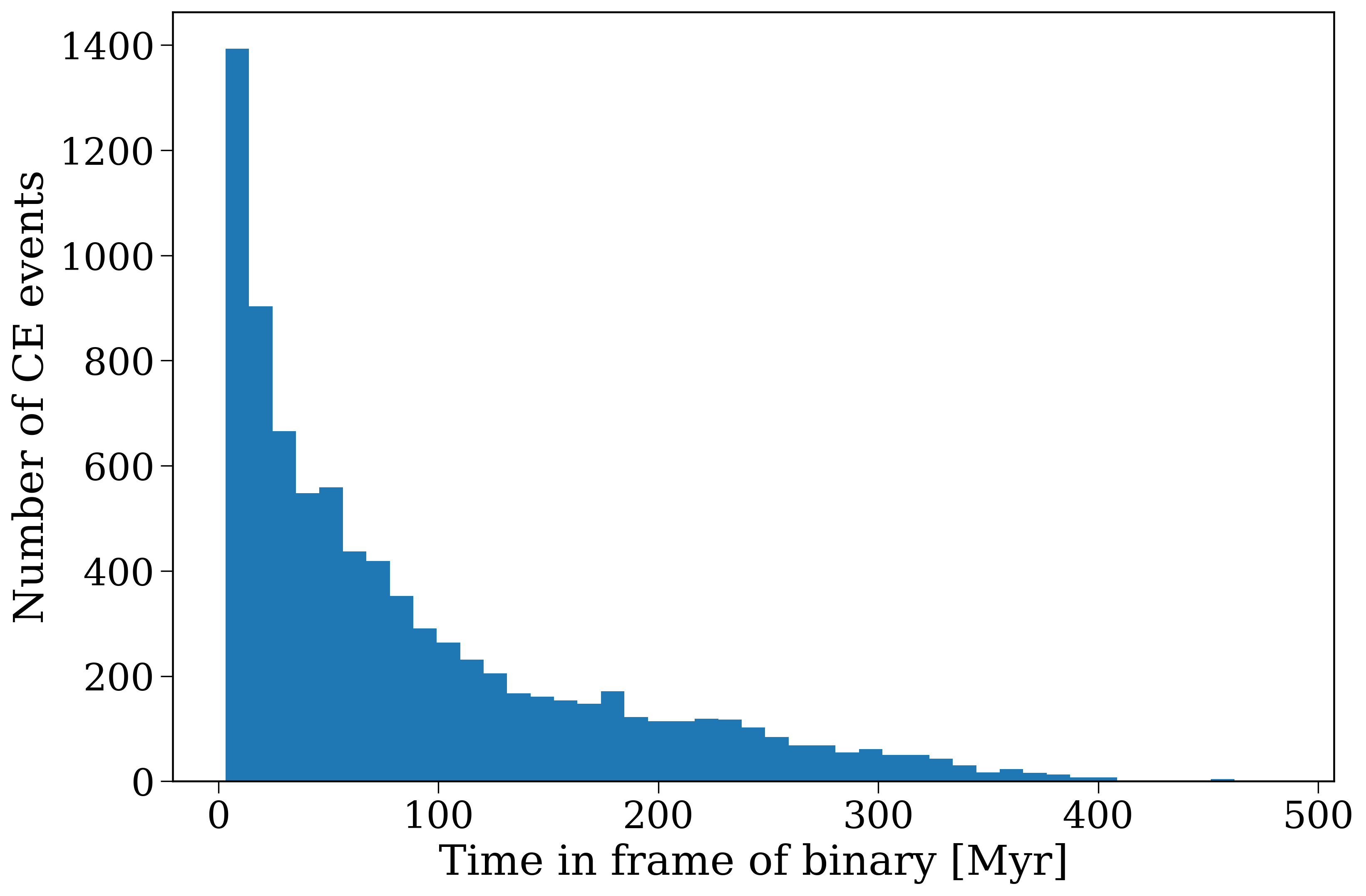
Distribution of common-envelope event times in the frame of the binary.

A common-envelope event occurs when a star overflows its Roche lobe in an unstable manner. So if we simplify a little, the timing is mainly driven by:

1. when the star evolves off the main sequence and expands

2. how far apart the stars are

3. how large the Roche lobe is (which depends on the mass ratio).

It’s a little more complicated in practice, since the typically stability of mass transfer is different depending on the evolutionary stage of the star when it overflows its Roche lobe (case A, B, or C).

But in general, we would expect common-envelope events to occur sooner for higher mass stars since those will expand sooner. We would also expect common-envelope events to be more common and to occur faster for shorter initial orbital periods.

Task 3.3

Now compute the timing of these common-envelope events in the frame of the galaxy. What drives the distribution of timing of these common-envelope events on Galactic timescale?

Hint

Remember that you can convert the common-envelope event times to the galactic frame using the same method as for the common-envelope events.

The conversion is given by:

\[t_{\rm gal} = t_{\rm present} - \tau + t_{\rm ce}\]

where \(t_{\rm ce}\) is the time of the common-envelope event in the binary frame and \(t_{\rm present}\) is the present day time in the galaxy (which is 12 Gyr by default, but is stored in the max_ev_time attribute).

Click here to reveal the answer

# get the bin_nums of the common-envelope events
ce_bin_nums = ce_rows["bin_num"]

# get the indices of these bin_nums in the p.bin_nums array
ce_indices = np.searchsorted(p.bin_nums, ce_bin_nums)

# use these indices to get tau
ce_tau = p.initial_galaxy.tau[ce_indices]

# compute the galactic times
ce_t_gal = p.max_ev_time - ce_tau + ce_rows["tphys"].values * u.Myr

fig, ax = plt.subplots()
ax.hist(ce_t_gal.to(u.Gyr).value, bins="auto")
ax.set(
    xlabel="Age of Milky Way [Gyr]",
    ylabel="Number of CE events",
)
plt.show()

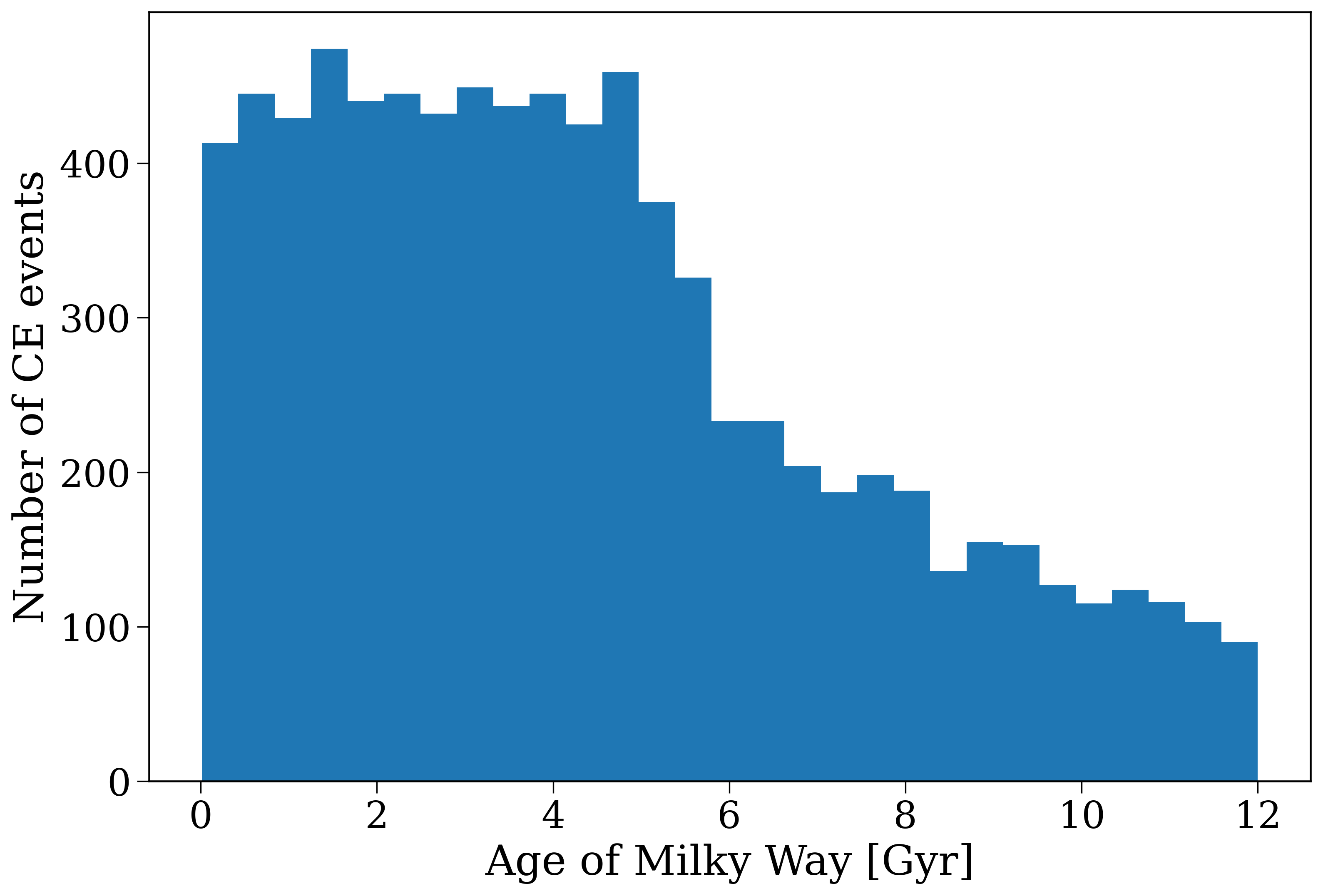
Distribution of common-envelope event times in the frame of the galaxy.

The timing in the frame of the binary is relatively short on the scale of the galaxy (most occur within 100 Myr, see earlier plot). So the main driver of the distribution on galactic timescales is the star formation history of the galaxy. In this case, we have a Milky Way-like SFH, which means that most stars (and therefore most common-envelope events) occur early on in the galaxy’s history, which is why we see a peak at early times in the histogram.

Task 3.4

Last but not least, let’s find the positions of these common-envelope events in the galaxy!

Follow the same method as above to find the positions of these common-envelope events in the galaxy and make a plot of these positions like the one above, though \(x\) and \(y\) limits of 20 kpc and \(z\) limits of 5 kpc should work well for this. (Why do you think these limits are smaller than for the supernovae plot above?)

Hint

Remember that, by definition, the common-envelope event occurs at the same location for both stars, so you can simply use the regular orbits array to find the positions of these events.

Click here to reveal the answer

ce_positions = np.zeros((len(ce_rows), 3)) * u.kpc

# go through each of the common-envelope events
for i in range(len(ce_indices)):
    # find the corresponding orbit
    ce_orbit = p.orbits[ce_indices[i]]

    # compute the last timestep where orbit.t is less than ce_t_gal[i]
    closest_time_index = np.where(ce_orbit.t < ce_t_gal[i])[0][-1]

    # get the position of the binary at this time
    ce_positions[i] = ce_orbit.pos.xyz[:, closest_time_index]

fig, axes = plt.subplots(2, 1, figsize=(8, 9), gridspec_kw={"height_ratios": [1, 4]})

XMAX = 20
ZMAX = 5

axes[0].scatter(
    ce_positions[:, 0], ce_positions[:, 2],
    c=ce_t_gal.to(u.Gyr).value, s=5,
    cmap="magma", vmin=0, vmax=12
)
axes[0].set(
    ylabel="$z$ [kpc]",
    xlim=(-XMAX, XMAX),
    ylim=(-ZMAX, ZMAX),
    aspect="equal",
)

axes[1].scatter(
    ce_positions[:, 0], ce_positions[:, 1],
    c=ce_t_gal.to(u.Gyr).value, s=5,
    cmap="magma", vmin=0, vmax=12
)
axes[1].set(
    xlabel="Galactocentric $x$ [kpc]",
    ylabel="Galactocentric $y$ [kpc]",
    xlim=(-XMAX, XMAX),
    ylim=(-XMAX, XMAX),
    aspect="equal",
)

fig.colorbar(axes[0].collections[0], ax=axes, label="Age of Milky Way at CE [Gyr]")

plt.show()

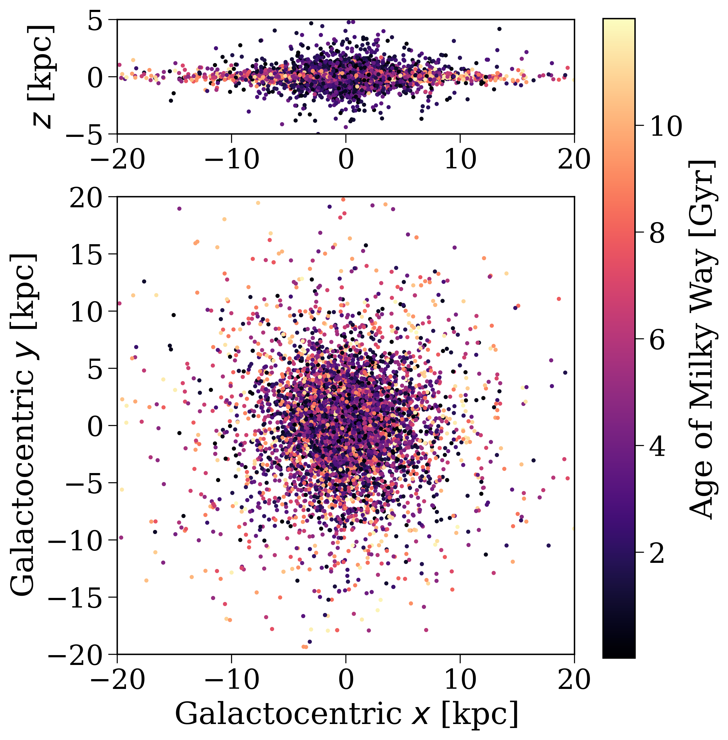
Positions of common-envelope events in the galaxy. The colour indicates the age of the Milky Way at which the common-envelope event occurs.