Part 4: Varying our assumptions#
In this final part, we are going to do what any good user of population synthesis codes does — vary our assumptions and see how it changes our results!
Tip
For a full list of the initial conditions and binary physics variations you could use, check out this page of the COSMIC docs. Specifically, the sampling parameters are found here and the binary physics parameters are here.
Why do we use population synthesis codes?#
We’ve seen that MESA or more detailed codes can more accurately model the evolution of stars - but they are too computationally expensive to run for large populations of binaries. On the other hand, cogsworth is much faster, but it relies on a lot of assumptions and approximations to get that speed. So we need to be careful when using it to make sure that our results aren’t just a consequence of some particular assumption we made. By varying our assumptions and seeing how it changes our results, we can get a better sense of which assumptions are most important for the questions we’re trying to answer, and which ones we can be less concerned about.
Collaborative variations#
This is blatant copying of EB’s idea for a collaborative activity, but I thought it would be fun to do something like this in the lab!
Instead of the full lab which may be too long, inspired by EB’s session on Tuesday, I thought it could be fun to do something collaborative. If you’re participating live, I have hopefully handed to you a slip of paper with a particular physics setting to try. It will say something like
“alpha1” = 0.1
Your task is to
Find out what this parameter means and think about how it might impact binary evolution (you’re going to want to look through
COSMIC’s documentation to find this out!)Create a fiducial population that uses default settings
Re-run the fiducial population with the parameter on your slip of paper changed to the value I gave you
Use the function below to get some basic summary statistics about the population and see what changed - does it make sense?
Put your values into the shared spreadsheet linked above, check out the plots on the second sheet.
Example#
You can use the code below as a template for your variation. Just copy and paste it into your notebook, and then change the part that says “CHANGE THIS TO YOUR SETTING(S)” to whatever setting you have on your slip of paper. You might have more than one setting, just do each on its own line.
import cogsworth

# sample a fiducial population
fiducial = cogsworth.pop.Population(
    n_binaries=10_000,
    use_default_BSE_settings=True,
    final_kstar1=[13, 14],
)
fiducial.sample_initial_binaries()

# copy to a varied population
varied = fiducial.copy()

# ------------------------------------------
# ----- CHANGE THIS TO YOUR SETTING(S) -----
varied.BSE_settings["alpha1"] = 0.1
# ------------------------------------------

# run stellar evolution in both cases
fiducial.perform_stellar_evolution()
varied.perform_stellar_evolution()

def get_population_stats(pop):
    sn_times = pop.bpp[pop.bpp["evol_type"].isin([15, 16])]["tphys"]
    disruption_fraction = pop.disrupted.sum() / len(pop)
    bh_masses = np.concatenate([pop.final_bpp[pop.final_bpp["kstar_1"].isin([14])]["mass_1"],
                                pop.final_bpp[pop.final_bpp["kstar_2"].isin([14])]["mass_2"]])
    merger_fraction = (pop.final_bpp["sep"] == 0.0).sum() / len(pop)
    ce_per_msun = (pop.bpp["evol_type"] == 7).sum() / (pop.mass_singles + pop.mass_binaries)
    return {
        "disruption_fraction": disruption_fraction,
        "merger_fraction": merger_fraction,
        "ce_per_msun": ce_per_msun,
        "sn_per_msun": len(sn_times) / (pop.mass_singles + pop.mass_binaries),
        "sn_times": sn_times.describe().round(3),
        "bh_masses": pd.Series(bh_masses).describe().round(3),
    }

for pop, label in [(fiducial, "Fiducial"), (varied, "Varied")]:
    print(f"\n{label} Population Statistics:")
    print("-" * 30)
    stats = get_population_stats(pop)
    for key, value in stats.items():
        print(f"{key}: {np.round(value, 3) if isinstance(value, (int, float)) else value}")
Demo#
Let’s start by quickly creating a template population to use for our variations. At first, let’s just sample the binaries but not do any evolution yet. This will make it easy to use the same initial population for all of our variations, so that we can isolate the impact of changing our assumptions about the physics.
import cogsworth

template = cogsworth.pop.Population(
    n_binaries=10_000,
    use_default_BSE_settings=True,
    final_kstar1=[13, 14],
    final_kstar2=[13, 14],
)
template.sample_initial_binaries()
We can then copy this template and use it to run a fiducial population.
fiducial = template.copy()
fiducial.perform_stellar_evolution()
fiducial.perform_galactic_evolution()
Note
Notice that I didn’t do fiducial.create_population() here. This is because I want to have the same initial population for all of my variations, so I just copied the template and then ran the evolution steps separately.
Now let’s consider some different assumptions that we could vary.
Initial population distributions#
cogsworth makes some default assumptions about the initial population distributions. For example, it assumes you want to use an IMF following Kroupa 2001 and the initial orbital period distribution from Sana+2012. You can change these assumptions by changing the parameters in sampling_params in the Population constructor.
Let’s make a copy of our population and change the orbital period distribution to a custom power law distribution.
# copy the old population
diff_porb = template.copy()

# update sampling parameters and re-run
diff_porb.sampling_params["porb_model"] = {'min': 0.15, 'max': 5.5, 'slope': 0.5}
diff_porb.create_population()
Now we can compare the initial orbital period distributions of these two populations.
fig, ax = plt.subplots()

bins = np.logspace(0.15, 5.5, 30)
ax.hist(fiducial.initial_binaries["porb"], bins=bins, label="Sana+2012")
ax.hist(diff_porb.initial_binaries["porb"], bins=bins, label="Custom power law", alpha=0.7)
ax.set(
    xscale="log",
    xlabel="Initial orbital period [days]",
    ylabel="Number of binaries",
)
ax.legend()
plt.show()
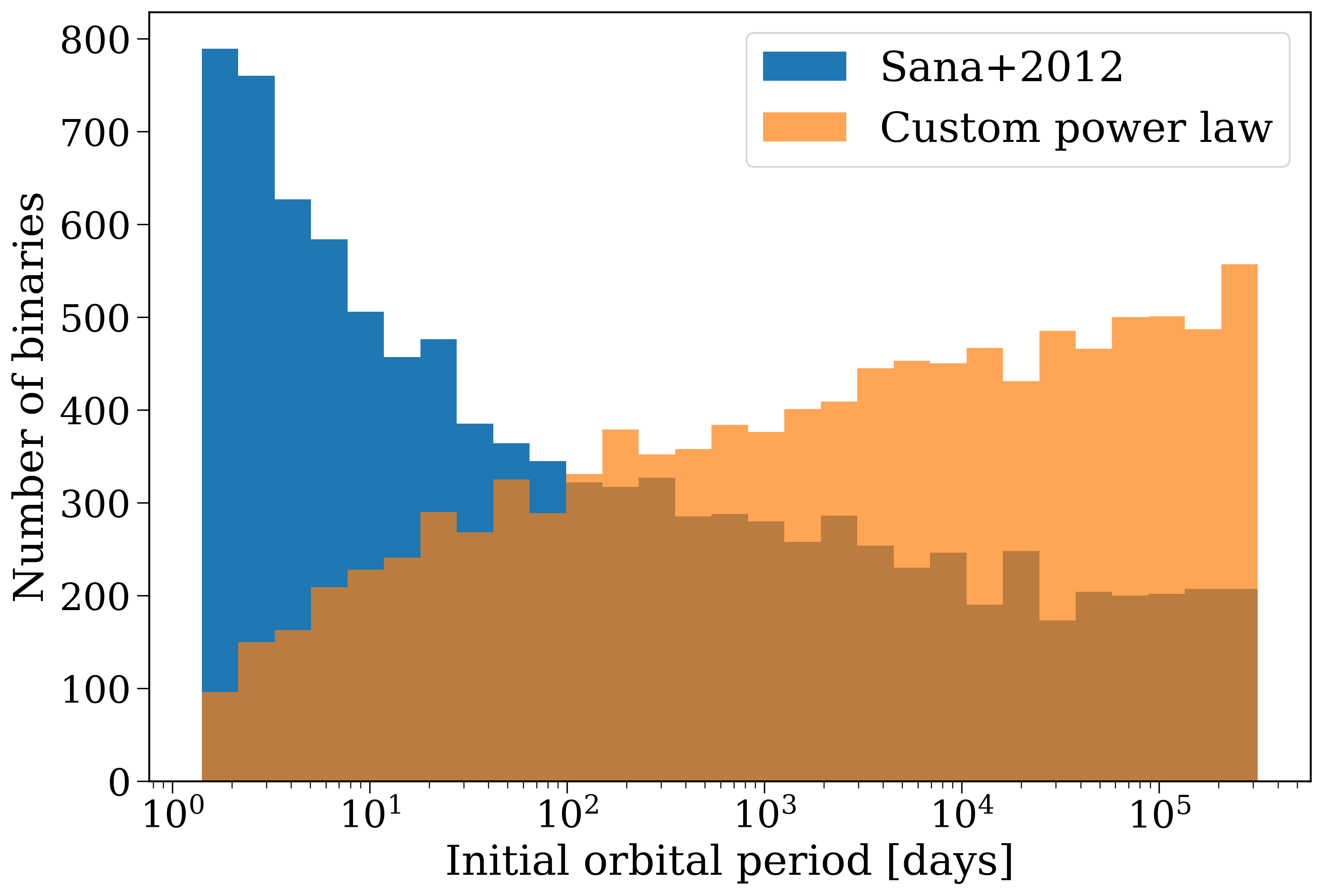
The initial orbital period distribution for the two populations.#
One can imagine that this change in the initial orbital period distribution could have a significant impact on the properties of the binary population at later times. Let’s see how it changes the number of mergers that occur in our population.
Question for you
Before looking at the results, can you predict how the rate of mergers will change when we switch from the Sana+2012 distribution to our custom power law distribution?
for pop, label in [(fiducial, "Sana+2012"), (diff_porb, "Custom power law")]:
    n_mergers = (pop.final_bpp["sep"] == 0.0).sum()
    print(f"Number of mergers with {label} porb distribution:", n_mergers)
Binary physics settings#
There’s also a lot of uncertainty in the physics of binary interactions. It’s therefore important that we vary our assumptions about these interactions to see how they impact our results. For example, we could change the common envelope efficiency parameter, or vary the strength of supernova natal kicks.
Let’s make a copy of our template population, but alter the strength of supernova natal kicks.
weak_kick = template.copy()
weak_kick.BSE_settings["sigma"] = 20  # km/s
weak_kick.perform_stellar_evolution()
weak_kick.perform_galactic_evolution()
By decreasing the strength of supernova natal kicks, it’s much less likely that binaries will be disrupted by supernovae. Let’s check that we’re getting fewer disruptions in this population compared to our fiducial population.
for pop, label in [(fiducial, "Fiducial"), (weak_kick, "Weak kicks")]:
    n_disrupted = pop.disrupted.sum()
    print(f"Number of disrupted binaries with {label}:", n_disrupted)
Bonus task
Try finding a binary that disrupts in the fiducial population but not in the weak kick population. Plot the orbit of this binary in both populations and see how the different kick strengths lead to different outcomes.
Click here to reveal the answer
fid_dis_nums = fiducial.bin_nums[fiducial.disrupted]
weak_dis_nums = weak_kick.bin_nums[weak_kick.disrupted]

# find one that is disrupted in fiducial but not in weak_kick
example = weak_kick.bin_nums[
    np.isin(weak_kick.bin_nums, fid_dis_nums)
    & ~np.isin(weak_kick.bin_nums, weak_dis_nums)
][0]

# plot both orbits together to see the difference
fig, axes = fiducial.plot_orbit(example, show=False)
weak_kick.plot_orbit(example, fig=fig, axes=axes, show_legend=False)

# perhaps try changing t_max to look at earlier times?
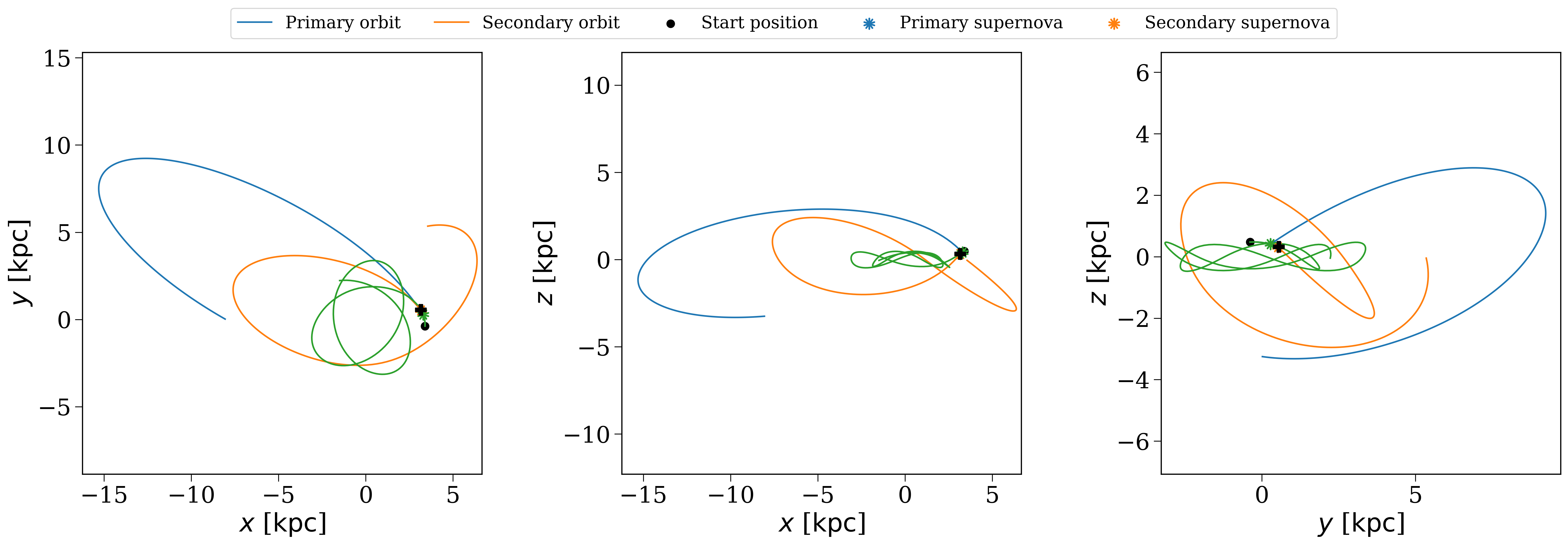
The orbit of a binary that disrupts in the fiducial population but not in the weak kick population.#
Galactic potential#
Finally, we could also vary the potential of the galaxy that we are integrating through. In this case, we don’t need to repeat the stellar evolution step, since the galactic potential doesn’t impact the binary interactions (or at least, we are assuming that).
Let’s create a new potential that’s an NFW profile with \(M_{\rm halo} = 10^{12} M_\odot\).
import gala.potential as gp

nfw = gp.NFWPotential(mhalo=1e12 * u.Msun, r_s=15.63 * u.kpc)

nfw_pop = fiducial.copy()
nfw_pop.galactic_potential = nfw
nfw_pop.perform_galactic_evolution()
Now let’s compare the orbit of a random binary that disrupts.
disrupted_num = fiducial.bin_nums[fiducial.disrupted][0]
for pop in [fiducial, nfw_pop]:
    pop.plot_orbit(disrupted_num, t_max=2000 * u.Myr)
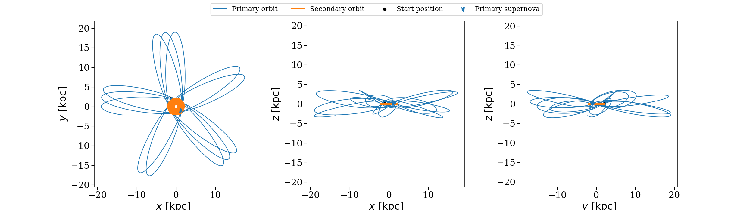
The orbit of a binary that disrupts in the fiducial population, evolved through the fiducial potential.#
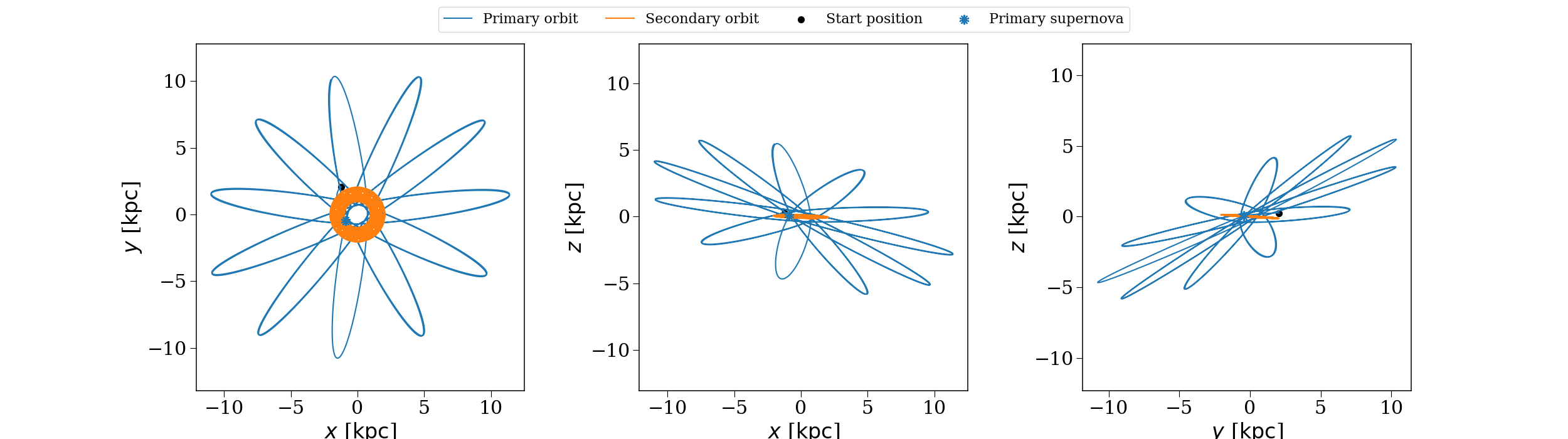
The same binary as the previous figure, but evolved through the NFW potential we created.#
Tasks#
You’ll not have time to do all of these tasks in the lab, so just pick whichever one looks more interesting to you (and no one’s stopping you doing the others later!).
The overall goal of these tasks is to explore how varying different assumptions changes the properties of the supernovae in the population. You can pick what you’re most interested in varying.
Task 4.1.1
Choose an initial condition to vary! Your full range of options is given here in the COSMIC docs.
Some inspiration for you:
You could try one of the other built-in initial orbital period distributions?
How does making the initial population entirely circular change things?
What if you set the minimum mass ratio to a larger value like 0.5?
Task 4.1.2
Create a template population and then make two copies of it. For one copy, your “fiducial” simulation, just call fiducial.create_population() to create the population and then evolve it.
For the other copy, change one of the sampling parameters like how we did above, and then re-run the sampling step and the evolution steps.
Make a plot of the initial distribution that you changed for both populations to check that it changed in the way you expected.
Hint
You can change the sampling parameters by updating YOURPOPULATION.sampling_params. You can access the initial binaries with YOURPOPULATION.initial_binaries after you run the sampling step.
Task 4.1.3
Use your code from Part 3 to get the timing and location of all supernovae in both populations. How do the supernova properties change when you change the initial conditions?
Task 4.2.1
Choose a binary physics assumption to vary! Your full range of options is given here in the COSMIC documentation.
Some inspiration for you:
Perhaps you could make common-envelopes 10x more efficient (
alpha1 = 10)?What if you make stable mass transfer always nonconservative (
acc_lim = 0)?Or maybe change how angular momentum is lost during Roche-lobe overflow at super-Eddington mass transfer rates? (
gamma)?
Task 4.2.2
Create a template population and then make two copies of it. For one copy, your “fiducial” simulation, just call fiducial.create_population() to create the population and then evolve it.
For the other copy, change one of the binary physics parameters like how we did above, and then run just the stellar evolution and galactic evolution steps (be careful not to do the sampling or you’ll get a different initial population!).
Pick a random binary in both populations and plot a cartoon of its evolution in both cases. Does it change how you would expect?
Hint
You can change the binary physics parameters by updating YOURPOPULATION.BSE_settings. You can plot the cartoon of a binary’s evolution with YOURPOPULATION.plot_cartoon(BINNUM).
Make sure you pick a random binary that experiences the binary interaction that you are trying to change! For example, if you’re changing the common envelope efficiency, make sure to pick a binary that actually goes through a common envelope phase to see a difference.
Task 4.2.3
Use your code from Part 3 to get the timing and location of all supernovae in both populations. How do the supernova properties change when you change the binary physics assumptions?
Task 4.3.1
Try creating a different galactic potential and evolving your population through it! You can use any of the potentials implemented in gala, but I’d probably recommend an NFW potential or a Miyamoto-Nagai potential for this task, with masses similar to the Milky Way.
Task 4.3.2
Create a template population and then make two copies of it. For one copy, your “fiducial” simulation, just call fiducial.create_population() to create the population and then evolve it.
For the other copy, update the potential like how we did above, and then run just the galactic evolution steps (be careful not to do the sampling or stellar evolution or you’ll get a different initial population!).
Pick a random binary in both populations and plot its galactic orbit. Does it change how you would expect?
Hint
You can change the galactic potential by updating YOURPOPULATION.galactic_potential. You can plot the orbit of a binary with YOURPOPULATION.plot_orbit(BINNUM).
Task 4.3.3
Use your code from Part 3 to get the timing and location of all supernovae in both populations. How do the supernova properties change when you change the galactic potential?